Visualizing BigQuery data in a Jupyter notebook

Setting up a Local Jupyter Environment

In this tutorial, you use a locally hosted Jupyter notebook. Complete the following steps to install Jupyter, set up authentication, and install the required Python libraries.

1. Run the following command in your terminal to install the latest version of the BigQuery Python client library, including the Pandas library, which is required for functions that use Pandas:

   pip install --upgrade google-cloud-bigquery[pandas]
   

2. Follow the installation instructions in the Jupyter documentation to install Jupyter.

3. Follow the instructions in the Getting started with authentication page to set up Application Default Credentials. You set up authentication by creating a service account and setting an environment variable.

Overview: Jupyter Notebooks

A notebook provides an environment to author and execute code. A notebook is essentially a source artifact, saved as a .ipynb file — it can contain descriptive text content, executable code blocks, and associated results (rendered as interactive HTML). Structurally, a notebook is a sequence of cells.

A cell is a block of input text that is evaluated to produce results. Cells can be of two types:

• Code cells: contain code to evaluate. Any outputs or results from executing the code are rendered immediately below the input code.

• Markdown cells: contain markdown text that is converted to HTML to produce headers, lists, and formatted text.

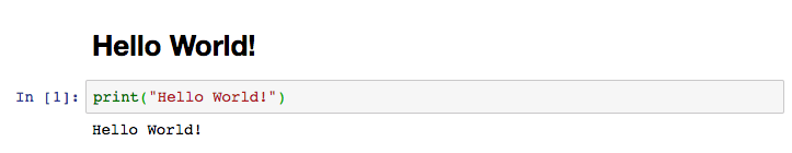
The screenshot below shows a markdown cell followed by a Python code cell. Note that the output of the Python cell is shown immediately below the code.

Each opened notebook is associated with a running session. In IPython, this is also referred to as a kernel. This session executes all the code entered within the notebook, and manages the state (variables, their values, functions and classes, and any existing Python modules you load).

Querying and visualizing BigQuery data

In this section of the tutorial, you create a Cloud Datalab notebook used to query and visualize data in BigQuery. You create visualizations using the data in the natality sample table. All queries in this tutorial are in standard SQL syntax.

To query and visualize BigQuery data using a Jupyter notebook:

1. If you haven't already started Jupyter, run the following command in your terminal:

   jupyter notebook
   

2. Jupyter should now be running and open in a browser window. In the Jupyter window, click the New button and select Python 2 or Python 3 to create a new Python notebook.

   

3. At the top of the page, click Untitled.

4. In the Rename notebook dialog, type a new name such as BigQuery tutorial, and then click Rename.

5. The BigQuery Python client library provides a magic command that allows you to run queries with minimal code. To load the magic commands from the client library, paste the following code into the first cell of the notebook.

   %load_ext google.cloud.bigquery

6. Run the command by clicking the Run button or with SHIFT + ENTER.

7. The BigQuery client library provides a cell magic, %%bigquery, which runs a SQL query and returns the results as a Pandas DataFrame. Enter the following into the next cell to return total births by year.

   %%bigquery
   SELECT
       source_year AS year,
       COUNT(is_male) AS birth_count
   FROM `bigquery-public-data.samples.natality`
   GROUP BY year
   ORDER BY year DESC
   LIMIT 15

8. Click Run.

9. The query results appear below the code cell.

   

10. In the next cell block, enter the following command to run the same query, but this time save the results to a new variable total_births, which is given as an argument to the %%bigquery. The results can then be used for further analysis and visualization.

    %%bigquery total_births
    SELECT
        source_year AS year,
        COUNT(is_male) AS birth_count
    FROM `bigquery-public-data.samples.natality`
    GROUP BY year
    ORDER BY year DESC
    LIMIT 15

11. Click Run.

12. Now you have a Pandas DataFrame saved to variable total_births, which is ready to plot. To prepare for plotting the query results, paste the following built-in magic command in the next cell to activate matplotlib, which is the library used by Pandas for plotting.

    %matplotlib inline

13. Click Run.

14. In the next cell, enter the following code to use the Pandas DataFrame.plot() method to visualize the query results as a bar chart. See the Pandas documentation to learn more about data visualization with Pandas.

    total_births.plot(kind='bar', x='year', y='birth_count');

15. Click Run.

16. The chart appears below the code block.

    

17. Next, paste the following query into the next cell to retrieve the number of births by weekday.

    %%bigquery births_by_weekday
    SELECT
        wday,
        SUM(CASE WHEN is_male THEN 1 ELSE 0 END) AS male_births,
        SUM(CASE WHEN is_male THEN 0 ELSE 1 END) AS female_births
    FROM `bigquery-public-data.samples.natality`
    WHERE wday IS NOT NULL
    GROUP BY wday
    ORDER BY wday ASC

    Because the wday (weekday) field allows null values, the query excludes records where wday is null.

18. Click Run.

19. In the next cell, enter the following code to visualize the query results using a line chart.

    births_by_weekday.plot(x='wday');

20. Click Run.

21. The chart appears below the code block. Notice the number of births dramatically decreases on Sunday (1) and Saturday (7).

    

22. Click File > Save and Checkpoint or click the save icon in the toolbar. Creating a checkpoint allows you to roll the notebook back to a previous state.

Pandas DataFrames

Magic commands allow you to use minimal syntax to interact with BigQuery. Behind the scenes, %%bigquery uses the BigQuery Python client library to run the given query, convert the results to a Pandas Dataframe, optionally save the results to a variable, and finally display the results. Using the BigQuery Python client library directly instead of through magic commands gives you more control over your queries and allows for more complex configurations. The library's integrations with Pandas enable you to combine the power of declarative SQL with imperative code (Python) to perform interesting data analysis, visualization, and transformation tasks.

Querying and visualizing BigQuery data using pandas DataFrames

In this section of the tutorial, you query and visualize data in BigQuery using pandas DataFrames. You use the BigQuery Python client library to query BigQuery data. You use the Pandas library to analyze data using DataFrames.

1. Type the following Python code into the next cell to import the BigQuery Python client library and initialize a client. The BigQuery client is used to send and receive messages from the BigQuery API.

   from google.cloud import bigquery
   client = bigquery.Client()

2. Click Run.

3. Use the Client.query() method to run a query. In the next cell, enter the following code to run a query to retrieve the annual count of plural births by plurality (2 for twins, 3 for triplets, and so on).

   sql = """
   SELECT
       plurality,
       COUNT(1) AS count,
       year
   FROM
       `bigquery-public-data.samples.natality`
   WHERE
       NOT IS_NAN(plurality) AND plurality > 1
   GROUP BY
       plurality, year
   ORDER BY
       count DESC
   """
   df = client.query(sql).to_dataframe()
   df.head()

4. Click Run.

5. To chart the query results in your DataFrame, insert the following code into the next cell to pivot the data and create a stacked bar chart of the count of plural births over time.

   pivot_table = df.pivot(index='year', columns='plurality', values='count')
   pivot_table.plot(kind='bar', stacked=True, figsize=(15, 7));

6. Click Run.

7. The chart appears below the code block.

   

8. In the next cell, enter the following query to retrieve the count of births by the number of gestation weeks.

   sql = """
   SELECT
       gestation_weeks,
       COUNT(1) AS count
   FROM
       `bigquery-public-data.samples.natality`
   WHERE
       NOT IS_NAN(gestation_weeks) AND gestation_weeks <> 99
   GROUP BY
       gestation_weeks
   ORDER BY
       gestation_weeks
   """
   df = client.query(sql).to_dataframe()

9. Click Run.

10. To chart the query results in your DataFrame, paste the following code in the next cell.

    ax = df.plot(kind='bar', x='gestation_weeks', y='count', figsize=(15,7))
    ax.set_title('Count of Births by Gestation Weeks')
    ax.set_xlabel('Gestation Weeks')
    ax.set_ylabel('Count');

11. Click Run.

12. The bar chart appears below the code block.